A photometric investigation of the galaxy cluster Abell 2666
1 Introduction
Amateur astronomy is experiencing a new golden age as specialized ccd cameras are becoming available and affordable. Amateur astrophotographers are collaborating with professionals on everything from variable star research to gamma ray burst studies. They are contributing important data and helping to increase our understanding of the universe around us. This paper details my attempt to familiarize myself with scientifically useful astronomical imaging using equipment accessible to a wide range of amateur astronomers, and internet-based astronomical catalogs.
The field of investigation is centered on the Abell 2666 galaxy cluster, in the constellation Pegasus at RA 23h 51m 22s, Dec 27d 10m 21s.
2 Equipment
All observing was done at the Galaxy Quest Observatory, owned by Jacob Gerritsen in Lincolnville, Maine, USA at 44 20.5° N 069 03.8° W using equipment graciously loaned by the owner. The telescope used for all the research image acquisition was a Televue NP-101 apochromatic refractor of the Nagler-Petzval design with a 101 mm aperture and 543 mm focal length mounted on an Astrophysics AP600GTO mount, and carefully polar aligned. The mount is attached to a sand-filled 12" pipe that is in turn bolted to a large 4' x 4' concrete block that has been inset into the ground.
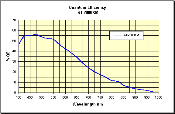
Figure 2.1 Spectral resopnse of the KAI-2001M CCD chip.
The imaging camera was an SBIG ST-2000XM anti-blooming camera with an internal TC-237 autoguider chip and cooled to -20 C. This camera has 7.4-micron square pixels in an 11.8 by 8.9 mm array. Mounted to the NP-101, it gives a 2.8 arcseconds/pixel image scale. Figure 1 shows the spectral response of the KAI-2001M CCD chip in this camera. It is clear from the graph that this camera is weighted heavily towards the blue end.
2.1 Software and astronomical catalogs
Maxim 1version 4.60 was used for all image acquisition and stacking and astrometry in conjunction with the Pinpoint2version 5.0 astrometric engine. The final stacked image was used as a background image in Cartes Du Ciel3 version 2.76c for galaxy identification. The internet visualization software, Aladin version 4 (Bonnarel et al 2000), was also used for object identification, with the SIMBAD dataset, from the CDS at Strasbourg, France, as well as the USNO-B (Monet et al 2003), GSC 2.3 (Spagna et al 2006), J/AJ/116/1529 (Hill & Oegerle 1998), and HYPERLEDA PGC (Paturel et al 2003) catalogs overlaid on the target area image. The Tycho2 catalog (Høg, E., et al 2000) provided magnitude reference data. Sextractor4version 2.5.0 was used to extract sources from the image.
3 Methods
3.1 Image acquisition and processing
Each sub-exposure is an auto-guided 300-second image. All images were acquired on the nights of 14 and 15 Oct. 2007. Each image was dithered via the autoguider between exposures. Autoguider exposure time was 2 seconds.Ten individual 300-second dark frames were exposed on October 15th with the camera mechanical shutter closed. These were sigma combined in Maxim DL into a master dark frame.
Ten bias frames were exposed on Oct. 15 with the mechanical shutter closed. These were combined into a master dark frame in Maxim DL.
Ten individual evening twilight flats were automatically scaled and sigma combined in Maxim DL on Oct. 15. The twilight sky conditions were such that I had some difficulty getting a good set of flats. There was a partly cloudy sky, so that I had to carefully time my flats between clouds. The flats were taken in an area of the sky just east of the zenith.
Flat field frames were bias corrected and combined into a master flat, then divided into each sub-exposure. Each sub-exposure was dark frame corrected and bias corrected in Maxim DL.
44 300-second images were plate-solved using Pinpoint and then astrometrically aligned and summed in Maxim DL for a total exposure of 13200 seconds.
3.2 Image post-processing and data reduction
The final image (Figure 2) was cropped to limit any edge of field distortion inherent in the telescope design. All magnitude estimates were done using this image. To enhance the overall visual appeal of the image, I imported the fits file into Photoshop and adjusted the curves and levels and applied a noise reduction filter (see Figure 3). For visual target identification, I modified the image by applying a mild low-pass filter, and a mild unsharp mask. The image was also inverted so that the background was white (see Figure 4).
I used Sextractor to extract objects from a filtered and sharpened version of figure 2 into a database with J2000 RA, Dec, and Best_Mag as columns. I then imported the object extraction database (OED) into Aladin and used the cross-match tool to determine which objects were within 5 arcseconds of a GSC 2.3 object. These cross-matched objects were then exported to a file with J200 RA, GSC 2.3 name, and distance from OED objects as columns. This cross-matched database (CMD) contains all the objects in the image that correspond to a GSC 2.3 object. The CMD was then compared to the GSC 2.3 catalog covering the image area, and all objects present in the CMD were flagged in the GSC 2.3 list. This entire procedure was replicated using USNO-B catalog data. Catalogs were provided by the Vizier query service (Ochsenbein et al 2000).
4 Results
4.1 Images
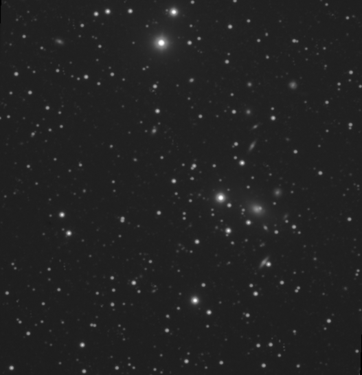
Figure 4.1: 13200 second calibrated and cropped image of the region around Abell 2666 (north is up, east is left).
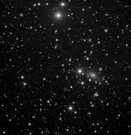
Figure 4.2: Enhanced image of the Abell 2666 region
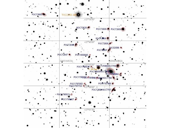
Figure 4: PGC Galaxies in Abell 2666 overlaid on deep field image
4.2 Magnitude estimates
In the field, the dimmest star detectable is listed in the USNO-B catalog as having a blue B1 magnitude of >20, and the brightest star, Tycho 2255-00345-1, is listed as having a visual magnitude of 8.08. See §5.4 for details about measuring magnitudes from the image.
4.3 Object distribution
4.3.1 Galaxies
Reaching beyond 18th magnitude, all 24 of the PGC galaxies comprising Abell 2666 listed in Table 1 were visible.
Table 4.1: PGC Objects in Figure 4
|
RA |
dec |
Name |
Alt Name |
Class |
Dim 1 |
Dim 2 |
B1 Mag |
Obs. Mag. |
Surface Brightness |
Radial Vel. |
|
23h50m47.47s |
+27°17'16.3" |
PGC0072600 |
|
Sbc |
0.7 |
0.6' |
14.98 |
|
13.85 |
7992 |
|
23h50m49.20s |
+27°13'35.5" |
PGC0072586 |
|
S? |
0.3 |
0.2' |
17.93 |
16.91 |
14.56 |
7573 |
|
23h50m49.81s |
+27°08'20.4" |
PGC1798869 |
|
|
0.6 |
0.3' |
17.34 |
|
15.01 |
|
|
23h50m52.22s |
+27°09'58.1" |
PGC0072596 |
NGC7765 |
S? |
0.7 |
0.5' |
15.68 |
|
14.33 |
7554 |
|
23h50m55.90s |
+27°07'34.7" |
PGC0072611 |
NGC7766 |
S? |
0.9 |
0.2' |
16.20 |
|
14.23 |
7938 |
|
23h50m56.51s |
+27°05'12.6" |
PGC0072601 |
NGC7767 |
S0-a |
1.1 |
0.3' |
14.52 |
|
12.86 |
8064 |
|
23h50m56.72s |
+27°06'26.6" |
PGC1797966 |
|
S? |
0.3 |
0.3' |
17.62 |
|
14.63 |
35297 |
|
23h50m58.27s |
+27°08'51.4" |
PGC0072605 |
NGC7768 |
E/cD |
1.5 |
1.0' |
13.28 |
|
13.4 |
8212 |
|
23h50m59.06s |
+27°14'27.4" |
PGC0072606 |
|
Sbc |
0.7 |
0.2' |
16.78 |
15.47 |
14.24 |
8142 |
|
23h51m00.00s |
+27°13'08.1" |
PGC0072607 |
|
Sb |
0.9 |
0.3' |
15.42 |
|
13.79 |
8313 |
|
23h51m00.79s |
+27°17'19.4" |
PGC0072609 |
|
S? |
0.4 |
0.4' |
16.38 |
|
14.05 |
9057 |
|
23h51m01.12s |
+27°15'27.5" |
PGC0072608 |
|
S? |
0.5 |
0.4' |
16.28 |
|
14.28 |
8634 |
|
23h51m10.94s |
+27°07'36.1" |
PGC1798514 |
|
S? |
0.3 |
0.2' |
17.54 |
|
14.33 |
32310 |
|
23h51m16.13s |
+27°09'49.5" |
PGC1799639 |
|
S? |
0.3 |
0.2' |
17.96 |
|
14.58 |
|
|
23h51m17.50s |
+27°12'10.4" |
PGC1800848 |
|
|
0.2 |
0.2' |
18.72 |
|
14.94 |
|
|
23h51m18.54s |
+27°17'36.8" |
PGC0072628 |
|
S? |
0.6 |
0.3' |
16.00 |
|
13.96 |
7915 |
|
23h51m18.94s |
+27°07'43.3" |
PGC1798583 |
|
|
0.3 |
0.2' |
18.68 |
|
14.97 |
|
|
23h51m22.10s |
+27°06'25.6" |
PGC1797950 |
|
S? |
0.2 |
0.2' |
18.14 |
|
14.69 |
35024 |
|
23h51m22.86s |
+27°05'58.8" |
PGC1797722 |
|
S? |
0.3 |
0.2' |
18.20 |
|
14.67 |
34878 |
|
23h51m29.99s |
+27°14'10.4" |
PGC0072640 |
|
E? |
0.6 |
0.3' |
15.78 |
14.72 |
13.8 |
8391 |
|
23h51m30.10s |
+27°03'16.6" |
PGC1796457 |
|
S? |
0.4 |
0.2' |
17.36 |
|
14.27 |
8427 |
|
23h51m34.06s |
+27°04'16.7" |
PGC1796915 |
|
|
0.2 |
0.2' |
18.61 |
|
14.96 |
8010 |
|
23h51m35.75s |
+27°12'12.3" |
PGC0072647 |
|
S? |
0.4 |
0.2' |
17.60 |
|
14.57 |
7771 |
|
23h51m58.90s |
+27°20'14.5" |
PGC0072665 |
|
Sb |
0.8 |
0.4' |
15.64 |
|
14.12 |
8126 |
4.3.2 Stars
There are only three stars brighter than 11th magnitude, including one pulsating variable, GR Peg, of spectral class M8, with a 71-day period as listed in the GCVS4.2 Catalog (Samus & Durlevich, 2004). A NASA ADS search of GR Peg yielded only one reference, "On the variable star GR Peg." by B. D. Pochinok (Astron. Tsirk., 944, 5-8 (1977)) with no abstract available.
4.3.3 Other objects
A query of the SIMBAD database indicates that there are a number of globular clusters associated with the central galaxy, NGC7768, although there is no evidence of them on the image. There are also two historical supernovas, neither of which was visible in the image. The NVSS survey (Condon, et al. 1998) at 1.4GHz detected the bright source 235147+271143 with no optical counterpart at 23 51 47.82 +27 11 43.0 with an integrated flux density of 23.3 mJy. It shows up as a large target (>19") in a NVSS image that covers the Figure 2 survey area.
5 Discussion
5.1 Abell 2666
Scodeggio et al. (1995) list the group's heliocentric radial velocity as 8134 msec-1. Table 1 lists radial velocities for some of the PGC galaxies in the cluster, and it is clear that most of those listed are all moving at speeds similar to that of the central galaxy, NGC 7768. Jordan et al. (2004) have studied the central galaxy in Abell 2666, NGC 7768, and found that it is a super-massive cD type galaxy. These are midway between galaxies and galaxy clusters in mass, and seem to be located at the dynamical and visual centers of galaxy clusters. Note, however, that there are four galaxies with a much higher radial velocity (>30,000 msec-1) (Hill & Oegerle 1998) that cannot possibly be dynamically linked to this NGC 7768 grouping.
Fanti et al (1982) note that there are no detectable radio source galaxies in the Abell 2666 group.
5.2 Source Extraction using Sextractor
After considerable experimentation (and much gnashing of teeth) with Sextractor parameters, 795 objects were extracted from the original fits file (Figure 2). When these extracted objects were overlaid on a filtered and sharpened image of the original fits image using Aladin, a careful visual inspection detected no spurious extractions. Each extraction had some visible object underlying it.
Listed below are the non-default Sextractor parameters that I arrived at to reduce spurious source extraction.
DEBLEND_NTHRESH 16
DEBLEND_MINCONT 0.00005
CLEAN Y
CLEAN_PARAM 5.0
SATUR_LEVEL 600000.0
MAG_ZEROPOINT 26.123467995
GAIN 0.61000014305114750
BACK_SIZE 64
BACK_FILTERSIZE 4
5.3 Source cross-matching with Aladin
Any extracted object less than 5 arcseconds (~2 pixels) from a catalog source was cross-matched to two different catalogs with Aladin. 728 of 795 (92%) of extracted objects were cross-matched to the USNO-B catalog objects covering the image area, and 669 of 795 (84%) were cross-matched to GSC 2.3 objects.
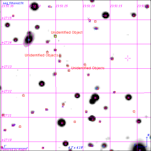
Figure 5.1: Representative screen shot of the overlaid catalog data on the filtered image
Figure 5.1 shows a representative screen clip of the Aladin image. The extracted objects are marked as red squares, and the blue plusses are cross-matched from the GSC 2.3 catalog and the magenta x's are USNO-B catalog cross-matches. Note that there are clearly visible objects that do not correspond to any catalog object. I searched all currently available Vizier catalogs without matching these visible objects. Given that my sub-exposures were all dithered, its unlikely that these represent hot pixels or other camera defects.
5.4 Estimating magnitude using Maxim DL
Maxim DL has a provision for magnitude calibration of the image. By measuring the intensity for a star of known magnitude, and entering the cataloged magnitude of the star, the astrometric information window will subsequently display the magnitude of the centroid under investigation.
Where possible, I have tried to find the blue magnitude for objects since the camera is much more sensitive to the blue end of the visual spectrum. Note that there are two blue magnitudes listed in the USNO-B catalog, B1 and B2. B1 filters are centered on 402.4 nm, and B2 on 448.0 nm, while B filters are centered between the two on 424.5 nm (Golay 1973). For the purposes of comparison, I am using B1 when it is present, and B2 if no B1 is present for the star in the catalog. Tycho2 uses a B filter. See Tables 2 and 3 for comparisons. See §5.6 for a discussion of the limitations of unfiltered magnitude comparisons.
5.4.1 Magnitude reference Star
I chose TYC2255-00275-1 as the magnitude reference star. In figure 1, it has an automatically scaled (by Maxim DL) intensity of 6.8597 in the 13200-second exposure. Its visual magnitude is listed in the Tycho-2 catalog as 10.78 and that is the value that I input into Maxim as the reference magnitude.
5.4.2 Magnitude comparison tables
Table 5.2, is a comparison of the HST GSC 1.1 (as reported by Pinpoint in Maxim DL) catalog magnitude and the observed magnitude (using Maxim DL) of several stars for a range of magnitudes.
Table 5.1: A sample of HST GSC 1.1 V magnitudes and B magnitudes from Tycho 2 and USNO-B in figure 4.1
|
Star |
RA |
Dec |
GSC 1.1 V Mag |
Cat. Blue Mag. |
Obs. Mag |
Blue magnitude source |
|
2255-00961 |
23h51m28.48s |
+27°08'35.4" |
13.81 |
14.56 |
13.94 |
USNO-B |
|
2255-01035 |
23h51m47.68s |
+27°22'07.1Ó |
13.05 |
13.47 |
13.10 |
USNO-B |
|
2255-01953 |
23h51m17.41s |
+27°02'38.1" |
10.53 |
11.9 |
11.35 |
Tycho 2 |
|
2255-00797 |
23h50m36.64s |
+27°01'13.9" |
13.85 |
14.17 |
13.90 |
USNO-B |
|
2255-00865 |
23h50m30.77s |
+27°21'51.1" |
15.00 |
15.53 |
15.52 |
USNO-B |
|
2255-00345 |
23h51m27.70s |
+27°20'09.8" |
8.08 |
10.50 |
10.13 |
Tycho 2 |
In Table 5.2, similar comparisons are made, but using the USNO-B catalog for the dimmer stars.
Table 5.2: A Sample of USNO-B Stellar Blue Magnitudes in Figure 4.1
|
Star |
RA |
Dec |
Cat. Blue Mag. |
Obs. Mag. |
Comments |
|
1170-0665246 |
23:52:07.6 |
+27:04:54.2 |
19.61 |
19.72 |
Left edge of image |
|
1171-0687537 |
23:51:08.2 |
+27:06:11.6 |
21.23 |
20.29 |
Near NGC7768 |
|
1172-0710155 |
23:50:32.6 |
+27:15:34.3 |
20.04 |
20.10 |
Right edge of image |
|
1172-0708723 |
23:50:45.4 |
+27:21:00.0 |
20.31 |
20.24 |
Top right corner |
|
1169-0640858 |
23:51:10.0 |
+26:58:59.1 |
20.13 |
19.53 |
Bottom edge of image |
As can seen from the tables, the observed magnitudes extracted using Maxim DL compare quite well to the blue magnitudes listed in the Tycho-2 and USNO-B catalogs.
Using the USNO-B catalog as a reference overlay, objects in the image down to magnitude 20+ can be seen.
5.4.3 Magnitude estimates of extended objects
It appears that Maxim DL is better at estimating the magnitude of stars than that of extended objects. Table 1 shows the observed magnitudes of some of the smaller PGC galaxies as extracted from Maxim DL. Note that the observed magnitudes are 1 magnitude brighter than the catalog blue magnitude.
Magnitudes for extended objects are not so useful as a predictor of how easily an object can be seen. The magnitude is an integration of the light intensity from the entire object: large dim objects will have a magnitude comparable to small brighter objects.
Surface brightness is a derived parameter that takes into account the magnitude and area of the object to give a value that can be used to determine the visibility of these extended objects. Surface Brightness, S = m + 2.5logA, where m is magnitude, and A is the area of the object in square arcseconds. Surface brightness values in Table 1 agree fairly well with the blue magnitudes listed.
5.5 Sextractor magnitude estimates
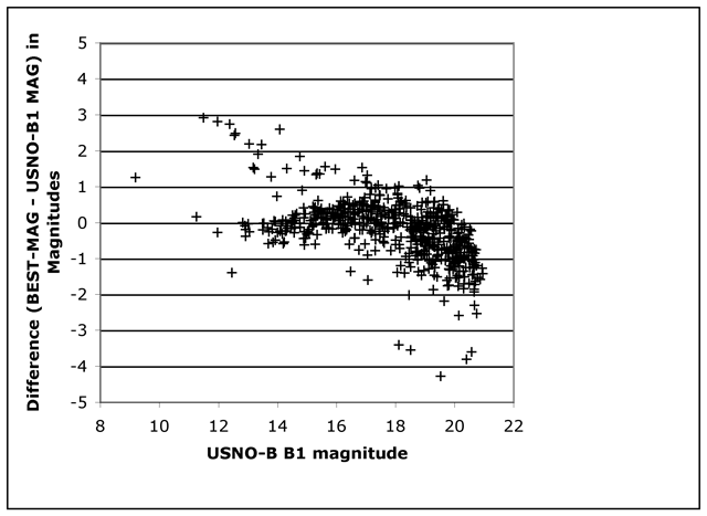
Figure 5.2: USNO-B blue mag vs. mag difference.
Even with careful gain and zero magnitude settings extracted from the fits header and corrected for total image integration time, Best_Mag values returned by Sextractor were offset from the USNO-B blue magnitude values. Figure 6 is a scatter plot of the difference between the corrected Best_Mag and USNO-B blue magnitude vs. USNO-B blue magnitude. Note that I used an average of B1 and B2 values as the blue magnitude value. I adjusted the correction factor experimentally to +4.6 to bring the bulk of the data to the zero offset line. With this offset applied to Best_Match values, there is a reasonable correlation to USNO-B blue magnitude values across a range of magnitudes from 14 to 18. Dimmer star magnitudes are underestimated by Sextractor. Perhaps more careful Sextractor parameter setting would yield more reliable Best_Mag data, but these particular data are of little value for extracted object magnitude estimates outside of this range.
5.6 Limitations of Unfiltered Images for Photometry
The image (Figure 4.1) was a sum of unfiltered sub-exposures, and as a result, object magnitudes are affected by the camera's spectral response. Without using photometric filters, comparison to photometric catalogs is difficult. The photometric magnitudes are calculated using filters that have a specific spectral response, and anyone choosing to do photometric magnitude estimates really needs to use filters with identical spectral response.
The standard filter set for photometry consists of five filters, Johnson U, Johnson B, Johnson V (yellow), Cousins R, and Cousins I5. Each of these filters limits transmission to a color pass-band. Images taken through one of these filters can be calibrated and compared directly with catalog magnitudes of the corresponding filter.
Color and therefore spectral class of a star can be determined by taking two separate images of the star with filters of adjacent bandpasses. The difference between the observed magnitude in each filtered image is called the color index.
The most commonly used index is B-V. Stars with a negative B-V index are blue and hot, and conversely, large positive B-V values correspond to cool, red stars. Vega is the zero magnitude standard for all the color bands, so in every color index, Vega's value is 0. Vega is a white star with spectral class A0.
Let's take a closer look at the brightest star in the image, Tycho 2255-345. The catalog B magnitude is listed at 8.175, and the V magnitude as 9.300 and a B-V index of .972 so this is a red star. I would expect Maxim to underestimate its visual magnitude because my camera's spectral response is weighted towards the blue end. Indeed, Maxim DL's photometric value for the star is 10.13. This example underscores the need for photometric filters for any study that requires accurate magnitude estimates.
5.7 Color distribution of extracted stars
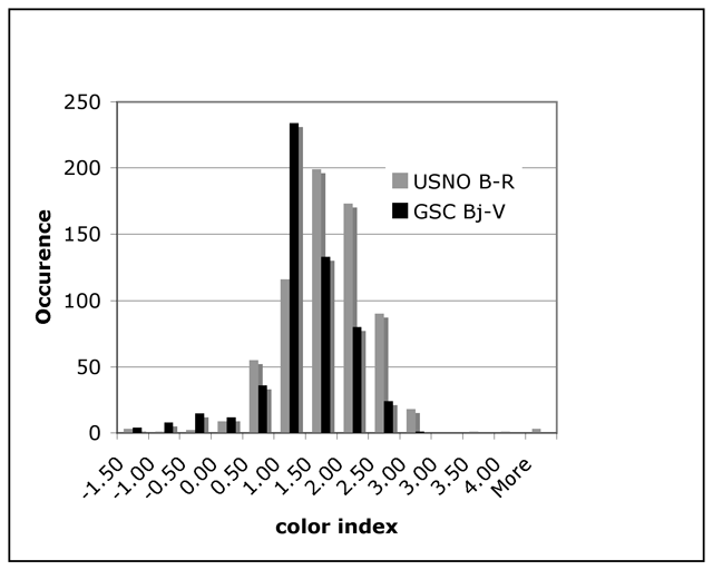
Figure 5.3: Color index of extracted stars
USNO-B data includes B and R data, while GSC2.3 includes Bj and V data. The Bj filter is similar to the B filter (Gullixson 1995). The Bj-V values are then approximately a B-V color index. Figure 7 is a histogram of the Bj-V color index of the GSC 2.3 extracted stars (where magnitude data is present), and the B-R index of the USNO-B extracted stars.
As can be seen from Figure 5.3, the Bj-V and B-R indices are skewed with respect to each other. Although the two indices are identical at 0, their numerical correlations to spectral class are different, as discussed below.
The USNO-B catalog lists blue and red magnitudes for many stars. There are two blue and two red entries (see §5.4). I have averaged the blue and the red magnitudes for each extracted star and then calculated the B-R value. B-R index values are an indication of the color of the star. Essentially, blue stars have negative values, white stars are 0 and red stars have positive values > 1.5. White stars of spectral class A0 have a B-R index value of 06. Our sun (spectral class G2) has a B-R index of 1.03 (Doressoundiram et al 2002). The B-R peak in Figure 7 is around 1.9, indicating that most of the stars in the sample are red. Very few stars with B-R less than 0 have been extracted.
B-V values are correlated to spectral class in in Table 5.1. The GSC 2.3 peak in Figure 7 is around 1.2, corresponding to red stars. There are few blue stars in the sample.
Table 5.3: B-V index and spectral type (Kaler 1989)
|
Color Index |
Spectral Type |
Approximate Color |
|
1.41 |
M0 |
Red |
|
0.82 |
K0 |
Orange |
|
0.59 |
G0 |
Yellow |
|
0.31 |
F0 |
Yellowish |
|
0.00 |
A0 |
White |
|
-0.29 |
B0 |
Blue |
Both color indices show many reddish and very few blue stars. If most of the stars detected in the image were from the galactic disk, we would expect a greater concentration of blue stars from the star forming regions in the spiral arms. Are the stars in the Figure 4.1 field population II stars from the halo of our galaxy? The field in Figure 4.1 is pointed well away from the galactic disk, so geometrically speaking, it is plausible that there are more halo stars along the line of sight than disk stars. Unfortunately, there is no coverage of the target area by the new RAVE study (Steinmetz et al 2006), which will provide radial velocity and metallicity data for several million stars when it is completed. If the radial velocity and metalilcity of the extracted sources were known, it would be a simple matter to see if these stars were population I or II. Population II stars would have greater radial velocities and lower metallicities.
5.8 Object detection percentage as a function of magnitude
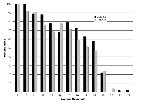
Figure 5.4: Percent of catalog objects detected as a function of magnitude
Figure 5.4 breaks down the cross-match percentage by average magnitude. Note that there are missing entries for all the magnitudes in both the USNO-B and the GSC 2.3 catalog, so in order to have a reference magnitude for histogram data, I have averaged all the magnitudes, regardless of how many are present. This may serve to skew the histogram in some way, but since the missing magnitudes seem to vary randomly, it is hoped that this does not change the histogram meaningfully. Limiting magnitude is reached when less than 75% of the sources in a catalog are detected (Pers. Comm Dr. Pamela L. Gay 2007) so for this image, that's magnitude 17. Detection percentage is somewhat dependent on careful tuning of Sextractor parameters, so its possible that more work there would have yielded higher limiting magnitude.
6 Conclusion
This paper has been an investigation into how to acquire, calibrate, process, and analyze a 3.7-hour CCD exposure of the region around the Abell 2666 galaxy cluster in the constellation Perseus.
Deep astrophotography is now within the reach of amateur astronomers. Using careful image calibration techniques, and stacking multiple images, relatively noise free high quality astronomical images can be obtained with consumer-grade CCD cameras available to the amateur astronomer. Anyone with a good mount, telescope and camera can get an image that reveals sources with magnitudes greater than 20. All that is needed is an investment in time, some cooperative weather, and a dedication to astronomy.
Using freely available software and astronomical catalogs, images can be astrometrically registered, and sources present on images can be extracted and cross-matched to catalogs. Magnitude estimates can be made and compared to catalog listed magnitudes. This availability of software and catalogs means that amateurs can participate in important scientific work in astronomy. These include variable star photometry, supernova detection, exoplanet orbit timing, minor planet detection, and many other areas. There is a growing pro-am collaboration in these and other areas, and it is to be hoped that as more amateurs learn techniques like those presented in this paper, this collaboration will continue to grow.
I wouldd like to thank Mr. Jacob Gerritsen of Camden, Maine, for the loan of his telescope and CCD Camera.
References
Bonnarel, F; Fernnique, P.; Boch, T.,2000, A&AS, 143, 3B
Condon, et al. 1998, AJ, 115, 1693
Doressoundiram, A. et al, 2002, AJ, 124, 2279D
Fanti, C., Fanti, R., Feretti, L., Ficarra, A., Gioia, I. M., Giovannini, G., 1982, A&A,105, 213
Golay, M, 1973, IAUS, 54, 275G
Gullixson, C. A., Boeshaar, P. C., Tyson, J. A., & Seitzer, P., 1995, ApJS, 99, 281G
Hill J.M.; Oegerle W.R., 1998, Astron. J. 116, 1529
Høg, E., et al. 2000, A&A, 355, L27
Kaler, James B, 1989, Stars and Their Spectra, Cambridge University Press, Cambridge.
Monet, et al, 2003, APj, 125, 984-993
Ochsenbein F., Bauer P., Marcout J., 2000, A&AS, 143, 221
Paturel et al, 2003, A&A,412, 45P
Samos, N.N; Durlevich, O. V., 2004, yCat, 2250, 0S
Scodeggio, M.; Solanes, J. M.; Giovanelli, R.; & Haynes, M. P.,1995, ApJ, 444, 63
Spagna et al, 2006, MmSAI, 77, 1166S
Steinmetz et al, 2006, arXiv:astro-ph/0606211v1
Jordan, Andres; Ct, Patrick; West, Michael J.; Marzke, Ronald O.; Minniti, Dante; Rejkuba, Marina, 2004, AJ, 127, 24-47
Footnotes
1 Diffraction Limited, 2007, Maxim DL Homepage, http://www.cyanogen.com/products/maxim_main.htm
2Denny, Robert, 2007, Pinpoint 5.0 Homepage, http://pinpoint.dc3.com
3Chevally, Patrick, 2006, Cartes du Ciel Homepage, http://www.stargazing.net/astropc/
4 Bertin, Emmanuel, 2006, Terapix, http://terapix.iap.fr/rubrique.php?id_rubrique=91/
5AAVSO CCD Observing Manual, 2007,http://www.aavso.org/observing/programs/ccd/manual/2.shtml#3
6The Columbia Encyclopedia, Sixth Edition Copyright 2004, Columbia University Press http://www.questia.com/PM.qst?a=o&d=101238295