An Investigation of M67's Color Magnitude Diagram
Abstract
Observing and constructing a color magnitude diagram of the open cluster M67 is within the capabilities of small aperture amateur telescopes using standard photometric filters and reasonably priced CCD cameras. I detail the process of acquiring and reducing photometric data using a variety of software tools. The resulting color magnitude diagram shows the turnoff from the main sequence that is in general accordance with the literature. Using a representative star, I calculate the age of the cluster.
1 Introduction
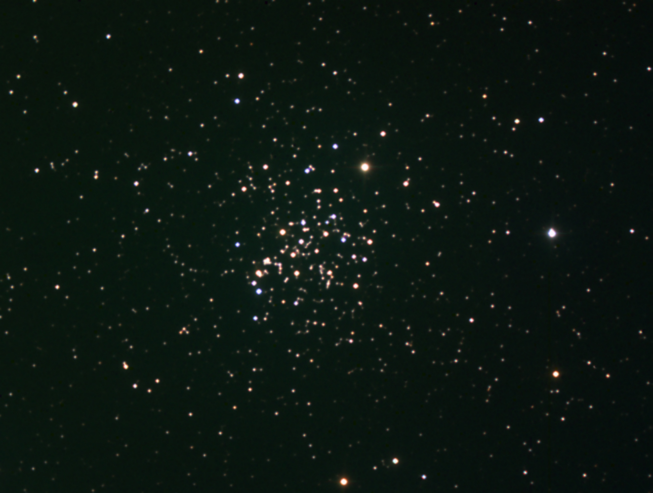
M67 is a rich, bright, open cluster in the constellation Cancer. It is visible to the naked eye from dark sky sites, and is visually comparable to many other rich clusters in small amateur telescopes. This visual similarity belies the cluster's unusual attribute: It is older than most other open clusters. Recent estimates (Dinescu et al 1995) put the cluster's age at 4 ± 0.5 Gyr. M67 has weathered the processes that have obliterated most other similar clusters because of its placement 405 pc above the galactic disk (Salaris et al 2004), well removed from most tidal effects. It has not been completely quiescent, since Fan et al. (1996) have shown that it is ovoid in shape, due to tidal stresses during its long life in orbit around the galactic core.
In this paper, I investigate the color magnitude diagram of M67 using data from images acquired with a 101mm aperture refractor and a thermoelectrically cooled ccd camera at the Double L Observatory in Camden, Maine through standard B and V photometric filters. I attempt to estimate the age of the cluster from main sequence turnoff magnitude.
2 Equipment and Location of Observations
Images were acquired at the Double L Observatory in Camden Maine, at 44 13 N latitude, 69 05 W longitude through a Televue1NP-101 Nagler-Petzval four element apochromatic refractor with an objective diameter of 101 mm. A Starlight Xpress2SXV-H9 thermoelectrically cooled CCD detector was coupled to the refractor with a set of Astrodon3 Schuler B and V filters in a filter wheel in the light path. The telescope is mounted on a carefully polar aligned German equatorial mount.
According to the Astrodon website, these filters are based on Bessel's 1992 modification to the Johnson-Cousins UVBRI filter standard and are used extensively by the AAVSO for variable star work.
The SXV-H9 is comprised of a Sony ICX285AL Exview HAD CCD chip with a 9 x 6.7 mm array of 6.45 μ m pixels that yields a 2.44 arcseconds/pixel image scale when coupled to the NP-101.
Image acquisition and calibration were done with Maxim D/L4using Russ Croman's RC Console Sigma Reject5algorithm for stacking.
3 Photometric observations and reductions
3.1 Image acquisition and reduction
36 30-second V- band images were exposed on 04-08-2008 00:38 UT (airmass 1.24) and sigma-reject median combined in Maxim D/L to provide the base V band image for further reduction.
Two different B-band images were constructed for this project. Image set one consists of five sigma-reject median combined 30-second sub-images all exposed on 04-08-2008. The midpoint UT time for these was 00:43 UTC at an airmass of 1.51. The second set consists of a sum of two 250-second sub-images exposed on 05-01-2008. The midpoint UT time was 00:57 at an airmass of 1.35
All sub-frames were bias and flat field corrected with a master bias consisting of 20 bias images, and a master flat consisting of 10 flat images exposed using a specially constructed light box with broad spectrum white LED's and a diffuser plate to ensure even illumination. See §4.1 for more on flat field image quality. No darks were taken since the detector has been measured by me to have a mean dark current of just 0.00159 e/pixel/sec at 0°C. The temperature during the observing run averaged 0°C and the camera cooled to -30°C, obviating the need for dark subtraction.
The V-band image was plate-solved using the Pinpoint6 astrometric engine and WCS astrometric data was appended to the FITS header.
3.2 Source extraction and catalog comparison
3.2.1 DAOFIND
With extensive help from Davis' (1994) DAOPHOT reference guide, I used the IRAF DAOPHOT photometry package for all photometry extraction. First, I ran DAOFIND on the V-band image to extract the pixel coordinates of the stars in the image. This is an iterative process that requires plotting the output of DAOFIND onto the image until only visible stars have been selected. IRAF includes several useful tools to do this: DISPLAY and TVMARK7. After careful adjustment of the parameters, DAOFIND extracted 456 sources from the center region of the image. This database was dumped into a simple text file using the TXDUMP command in IRAF. Each source was assigned a unique ID number by DAOFIND, and I used this ID as my master ID for all subsequent lists and databases.
3.2.2 ALADIN and CCXYMATCH
For the purpose of overlaying astronomical catalog data on images, the software package ALADIN (Bonnarel et al. 2000) is excellent. With access to virtually every astronomical catalog available online, catalog data can be displayed and overlaid on an image. Several catalogs can be displayed at once, and catalogs can be cross-matched to generate customized catalogs. Large all-sky catalog data can be retrieved for just the area covered by an image that includes WCS astrometric header data, and then exported to a file for use elsewhere.
I displayed the portion of the 2MASS survey (Skrutskie et al. 2006) coincident with my V-band image and exported it as a text file for use with the IRAF tool CCXYMATCH, to correlate pixel coordinates to J2000 RA and DEC positions as listed in the 2MASS survey. In order to use CCXYMATCH, a text file with user-defined tie points consisting of the RA and DEC values and corresponding pixel values for three easily identifiable stars.In order to match as many stars as possible, these stars should be selected near the edge of the image to make a rough equilateral triangle. By specifying two input files: WCS coordinate reference file and DAOFIND output, CCXYMATCH outputs a list of pixel coordinates matched to J2000 coordinates. Care must be taken to ensure that the line numbers output by CCXYMATCH are corrected to match the ID numbers output by DAOFIND. This new file needs to be edited to comply with ALADIN's data format, and then can be displayed as an overlay in ALADIN.
ALADIN has an additional powerful feature, the cross-match. Any two catalogs that share one parameter can be cross-matched to create a new catalog. I employed this cross-match feature many times to link my observed data to the literature.
3.3 Photometric measurement of extracted sources
IRAF includes the aperture photometry tool, PHOT, part of the DAOPHOT group. Using the coordinate file generated by DAOFIND, PHOT produces a list of magnitudes based on a set of input parameters.
PHOT takes a bit of getting used to, and I spent a great deal of time learning how to set the parameters to generate usable photometry data. It is important to set the background sky parameters correctly so that the background counts can be subtracted from the source counts. The background count value is determined by measuring counts in an annulus around a star. The user can set the radius and thickness of the annulus, the standard deviation of the background, and a photometric aperture inside of which the source counts are taken. I found that an aperture of 3 pixels and an inner sky radius of 11 pixels with a sky sampling width of 6 seemed to be the best settings for my data.
Statistically, the background counts will be more accurate if the annulus is wide (Howell 2006), but in a crowded field like M67, care must be taken to avoid contaminating the annulus by nearby stars. If any light from an adjacent star is included in the aperture, the sky background value will be too high. When the sky background is subtracted from the intensity of the star inside the aperture, the resultant intensity of the star will be underrepresented. This limits the accuracy of aperture photometry for star clusters. See §4.2.1 for a discussion.
All this photometry is dependent on a linear response of the CCD detector across a wide range of ADU counts. The SXV H9 is outstanding in this regard, and has been found by Warell (2006)8 to be within 1% of linear across most of its range. As long as ADU values are between 230 and 61000, this camera should be capable of attaining a photometric accuracy of 1%.
3.4 Photometric calibration
The values output by PHOT are raw instrument magnitudes. In order to place them on a standard scale, a general transformation equation is used,
Where M is the calibrated magnitude, m is the instrument magnitude, zp is the magnitude zero point offset, c is the color term, B is the calibrated B-band magnitude, V is the calibrated V-band magnitude, a is the extinction coefficient, and X is the airmass.
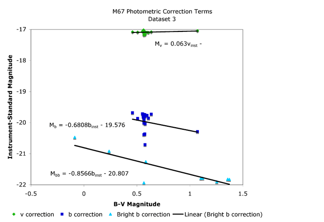
Figure 3.1 Dual image calibration graph
Since my standards are in my science field, the airmass term is not needed, so the two transformation equations (one for each color) become
and
Where the lower case b and v are the instrument raw magnitudes and the uppercase B and V are the calibrated magnitudes.
Note that there are no non-linear terms in the above transformation equations. Montgomery et al. (1993) (subsequently referred to as MMJ) do include a quadratic term in their transformation equations, but determining non-linear terms is beyond the scope of this project.
The astute reader will wonder how one can use the calibrated magnitudes on the right side of the equation to determine the calibrated magnitude on the left side. The solution involves using an estimate of the magnitudes and iteratively replacing the new output into subsequent equations until the solutions converge. See appendix 1 for a detailed explanation of this iterative technique.
I chose to use the B and V values presented by MMJ as my calibration standards. The photometry of this catalog was done in a highly rigorous manner, and included photometry from earlier studies. I used MMJ's list of 30 carefully selected calibration stars as my standards.
Careful inspection of instrument magnitudes vs. MMJ standard magnitudes in the B band showed a bifurcation at the bright end of the graph down to about 13th magnitude (figure 4.2). In order to further investigate this bifurcation I prepared three distinct B band datasets as outlined below:
Dataset 1: photometry from the 500-second sum image with a single set of blue calibration terms.
Dataset 2: photometry from the 500-second sum image with a dual set of calibration terms, blue and bright blue, with magnitude 13 as the dividing line. The calibration list was separated at magnitude 13, and two separate blue calibrations were done. The calibration terms for this set are derived from figure 3.1 which shows the least squares regression best-fit line for each standard set, v b and bright b. The slope of the line is the color term, and the y intercept is the zero point offset.
Dataset 3: photometry for stars dimmer than v magnitude 13 comes from the 500-second sum image, and for stars brighter than v magnitude 13 the photometry has been done using the 5 x 30 second median combined image with appropriate adjustment to the calibration terms. The shorter image stack eliminates the possibility of saturated brighter stars.
In each of the datasets, plots of B-band instrument magnitude vs. standard magnitude show a much larger scatter than the V-band data.. See §4.2.2 for further discussion.
3.5 Color Magnitude Diagrams
I present a color magnitude diagram for each of the three datasets outlined above. The B-band data is as follows: figure 3.2 from the single image single calibration photometry (Dataset 1); figure 3.3 with the single image dual calibration (Dataset 2); and figure 3.4 with dual image and dual calibration (Dataset 3). A supporting data table for Dataset 3 is included in the companion excel file, "M67 Dataset #3 data".
The V-band magnitudes of 459 stars from the central region of the image frame are plotted against their B-V color index. I have also plotted the MMJ data in red on figure 3.2 and 3.3.
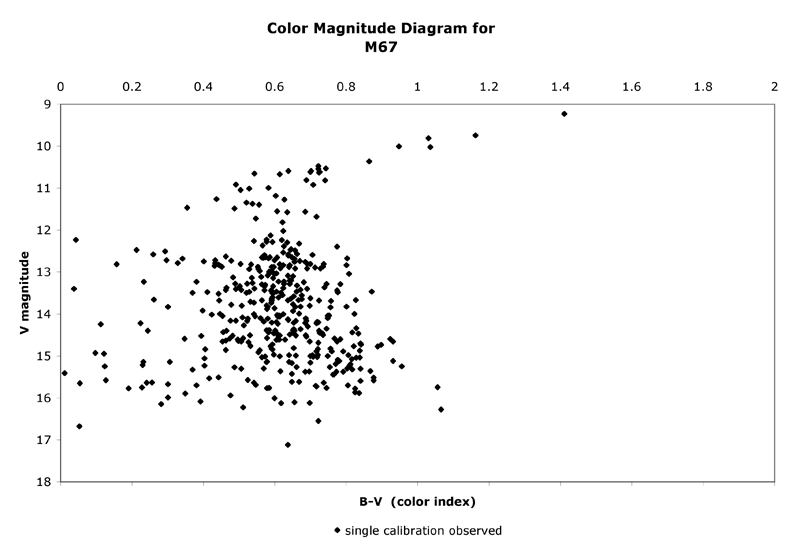
Figure 3.2 Dataset 1: Single calibration using photometry from 500-second image
Figure 3.3 Dataset 2: Dual calibration using photometry from 500-second image
Figure 3.4 Dataset 3: Dual calibration using photometry from two separate images
4 Discussion
4.1 Flat field quality
Since each science frame is divided by a bias-corrected flat field frame, final photometric accuracy depends on the quality of the flat field image. In order to determine the flatness of my flat fields, I acquired two sets of 10 flat frames. I rotated the light box by 90 degrees between sets. I median combined each set to obtain master images and divided the second master into the first master. By inspecting the histogram of this final image, I determined that the range of pixel values ranged from 30910 to 32294 in what appeared to be a Gaussian profile around a mean. That's a 4% variation in pixel values, so I conclude that my flat fields are flat only to ± 2%. This places a lower constraint on the accuracy of the photometry using this particular light box for flat field production.
4.2 Photometric data quality
4.2.1 V band data
The V band data was collected on a night of excellent transparency and good seeing. FWHM values are below 2 pixels (corresponding to 4.9 arcseconds), and the image exposure length of 30 seconds was optimal for obtaining ADU counts in the linear range of the detector.
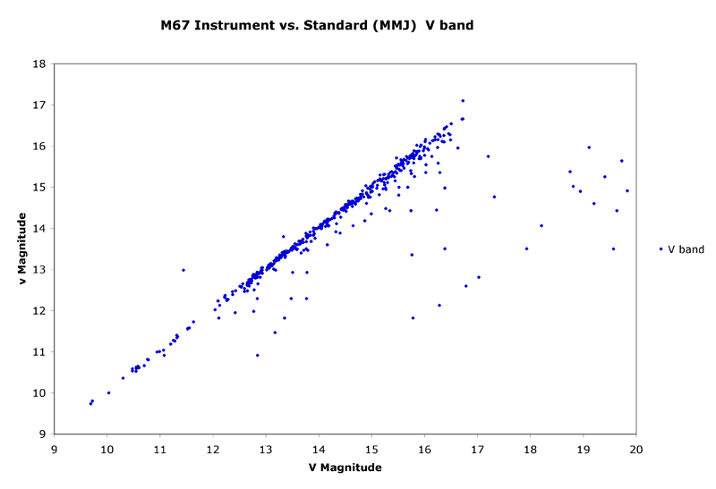
Figure 4.1 V band linearity
![]()
Then the mean of the error is 0.81% with σ = 3.32% and a skewness of 4.57.
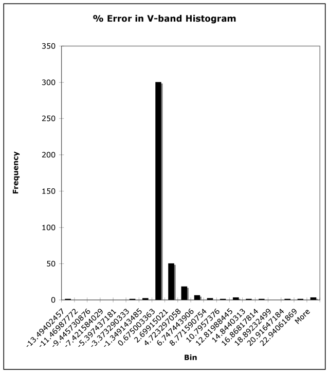
Figure 4.2 V band histogram
4.2.2 B band data
The B-band data from both images are not as good the V-band. That is not surprising given that the data comes from a stack of only 2 (or 5, for the case of the 30-second) images versus 36 for the V-band. Signal to noise ratio increases by the square root of the number of images stacked; the V band image has ~5 times the signal to noise of the 500-second B-band image. FHWM values are also higher than the V- band, averaging around 2.3 pixels. This is primarily due to the larger airmass for the 30-second images and due to the autoguiding errors that conspire to smear out the stars in the 500-second image.
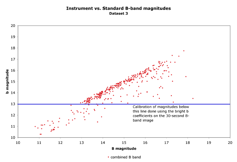
Figure 4.3 B band linearity
Figure 4.3 represents data with the dual calibration coefficients applied as discussed in §3.4. All three datasets exhibit the bright star bifurcation. Why this bifurcation is not present in the V band also is not well understood by me, but probably has to do with the poorer seeing and perhaps transparency of the B band image sky.
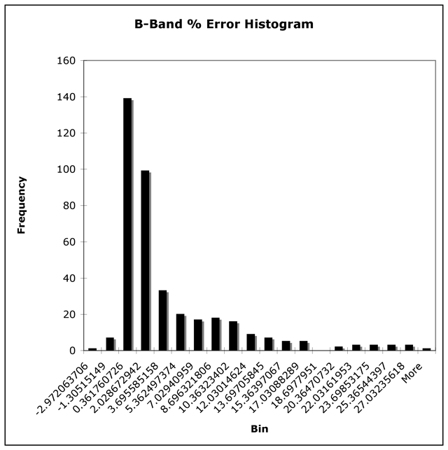
Figure 4.4 Dataset 2 B band histogram
Figure 4.4 shows the histogram of the Dataset 2 B-band % error. The mean was 3.32% with σ = 5.67 and skewness = 2.13. Here, there is even more systematic error than the V-band also skewed in the direction of instrument magnitudes being too low. Again, the cause is not understood.
4.2.3 Photometric accuracy
From the above rudimentary statistical analysis it would appear that my system is capable of attaining a photometric accuracy of ~ ± 3% on nights of excellent photometric quality. Accuracy degrades quickly if conditions are not ideal, as shown by the poorer quality B band data. Great care must be taken in generating calibration terms so that the error is not skewed away from 0. The primary sources of error seem to be flat field quality, atmospheric conditions, limitations of aperture photometry to crowded fields (as opposed to PSF fitting photometry) and detector linearity.
4.3 B band calibration
Having a priori knowledge of how an experiment should come out can lead to an inordinate amount of data manipulation to make sure that the outcome of the experiment is "right". I found myself spending dozens of hours adjusting PHOT parameters in order to get the observed data to correspond to the MMJ data (shown in red in figures 3.3 and 3.4).
This a priori> knowledge is what led to the application of two separate calibration schemes in order to displace the bright data to the right. Is this dual calibration scientifically justified? Using two separate images of different length exposures as is done in Dataset 3 is a common technique to avoid source saturation, but I suspect that a single image dual calibration scheme is not common. Note that there is a group of stars (the red giant clump?) in the MMJ data at V magnitude = 1.5 and B-V = 1.1 that seem to be represented in both Datasets 2 and 3. It is curious that the dual calibration used in Dataset 2 should overlay the MMJ data better than Dataset 3.
In the case of the blue (Mb) calibration graph (figure 3.1) there is so much scatter to the data that the least squares linear fitting does not represent a good model fit for the data. Removal of one of the calibration stars would alter the slope and intercept of the least squares fitted line. One could easily delete the calibration stars aiming for a fitting line that moves the data closer to the standard data. Nevertheless, without removing any calibration stars, the calibration terms seem to be quite good because the experimental data overlay the MMJ data well. Is the skew in the photometric accuracy due to the scatter in the calibration data? Probably, but further investigation is needed.
The bright blue (Mbb) calibration graph has very little scatter. The least squares regression line fits well with the data.
4.4 M67 characteristics
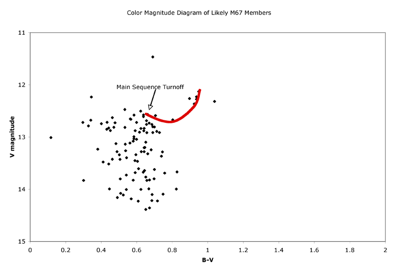
Figure 4.5 Dataset 2
The color magnitude diagram tells us a great deal about this cluster. Figures 3.3 and 3.4 show the main sequence (the tightening of stars along a diagonal line in the noisiest section of the diagram), the main sequence turnoff, the red giant branch, including several stars that may represent the red giant clump (Castellani et al. 1992) and finally the horizontal branch (of which there are very few example stars). Some of the scatter off the main sequence can be attributed to noise, but some is from background stars that are not members of the cluster. Additionally, since some of the stars are variable, their magnitudes will have changed since the MMJ results. By using membership probability estimates determined from proper motion studies (Sanders 1977), likely members (those with Sanders probabilities > 50%) are plotted in figure 4.5. Although the data are sparse, the main sequence turnoff can be clearly seen.
Notice the horizontal line of stars to the left of the main sequence in figures 3.3 and 3.4. These must all be stars that have turned off the main sequence, but because of poor B-band data quality, B-V values are noisy, and therefore their placement on the diagram is skewed.
4.4.1 Main sequence turnoff, distance and age determination
Regardless of the B-band calibration difficulties, the V-band data allows us to see the clear main sequence turnoff at V magnitude ~12.6. This is evident in figure 2.3. It is difficult to pick a B-V value that characterizes the main sequence at this magnitude due to the scatter: I'll pick a representative value of 0.6. For a star on the main sequence, this represents a G0 star with an absolute V-band magnitude, Mv of 4.4 (Binney and Merrifield 1998). Subtracting this from the MSTO V magnitude of 12.6, leads to an observed distance modulus of 8.2. This compares to the MMJ value of 9.6. We can use the equation
to calculate a distance to M67. In our case,
This value is about half of the MMJ value of 832 pc, confirming that the simplistic approach to determining the main sequence turnoff magnitude is fraught with error. Of course, equation 4.1 does not take into account any dust attenuation or considerations of metallicity of the cluster. MMJ states that adjustment to the transformation color terms must be made to account for reddening and metallicity, and both parameters are interrelated (Castellani et al. 1992). The lack of adjustment for reddening and metallicity is another source of magnitude error in my observational data, but inclusion of these terms is beyond the scope of this project.
From our color magnitude diagram, we can see that no stars brighter and bluer than G0 stars exist on the main sequence. These stars have already spent their hydrogen cores and have moved off the main sequence. Since G0 stars (similar to our sun) have a main sequence lifespan on the order of 5 Gyr, the cluster's age must be around that age, too. If it were older, the G0 stars would not be present on the main sequence, and if it were younger, there would be some F5 stars still present on the main sequence. More accurate age estimates require sophisticated isochronal line fitting. Isochrones can be generated from stellar evolution models, and overlaid on the observed data. By finding the best-fit curve, the age of the cluster can be determined. The entire process rests on the assumptions that went into the model, so there is some disparity of age in the literature based on the different models. Isochronal fitting is beyond the scope of this project.
5 Conclusion
Using low cost photometric filters, a commercially available CCD detector and a small aperture telescope, it is possible to construct a reasonably accurate color magnitude diagram of an open cluster. The resulting color magnitude diagram can be used to determine the distance, age, and general stellar characteristics of the cluster.
Care must be taken to acquire sufficient data to have high signal to noise ratio, and each frame must be reduced with dark and flat frames. Flat frames must be of high quality to avoid constraining overall photometric accuracy. Consideration must be given to atmospheric conditions, with preference given to nights of good seeing and unchanging transparency. Under ideal conditions, a photometric accuracy of ~ ± 3% is possible.
Appendix 1: Iterating color terms with Excel
Recall from the transformation equations (eq. 3.2 and 3.3) that the calibrated magnitudes are present in both sides of the equations. Clearly, if the un-calibrated magnitudes are substituted on the right side for B and V, the resultant magnitude will be incorrect.
I used an iterative technique in excel to have the solution converge to the final magnitude. The zero point offsets determined from the calibration routine are subtracted from the raw instrument magnitudes to get a base magnitude for each band. Figure A.1 shows the spreadsheet setup. Columns A and B are the instrument zero point magnitudes. Columns C and D are the first iteration, using the base magnitudes. Columns E and F are the second iterations. C_v and C_b are the V and B band color terms respectively. Note that the second v magnitude iteration uses the first b magnitude iteration and the second b magnitude iteration uses the first v magnitude iteration.

Figure A.1
The iteration should be continued until the values in subsequent iterations converge on an unchanging value at least for the first three decimal places. With my data, three iterations were sufficient for convergence.
References
Binney, J. and Merrifield, M ., 1993, Galactic Astronomy, Princeton University Press, Princeton, NJ
Bonnarel F.; Fernique P.; Bienayme O.; Egret D.; Genova F.; Louys M.; Ochsenbein F.; Wenger M.; Bartlett J.G., 2000A&AS, 143, 33B
Castellani, V., Chieffi, A., & Straniero, O., 1992, ApJS, 78, 517C
Davis, Lindsey E., 1994, A Reference Guide to the IRAF/DAOPHOT Package, NOAO, Tucson
Dinescu D. I., Demarque P., Guenther D. B., Pinsonneault M. H., 1995, AJ, 109, 2090
Fan, X., Burstein, D., Chen, J.-S., Zhu, J., Jiang, Z., Wu, H., 1996, AJ, 12, 628F
Montgomery K. A., Marschall L. A., Janes K. A. , 1993, AJ, 106, 181
Salaris,M.; Weiss,A.; Percival, S. M., 2004, A&A 414, 163
Sanders, W. L, 1977, A&AS, 27, 89
M.F. Skrutskie, R.M. Cutri, R. Stiening, M.D. Weinberg, S. Schneider, J.M. Carpenter, C. Beichman, R. Capps, T. Chester, J. Elias, J. Huchra, J. Liebert, C. Lonsdale, D.G. Monet, S. Price, P. Seitzer, T. Jarrett, J.D. Kirkpatrick, J. Gizis, E. Howard, T. Evans, J. Fowler, L. Fullmer, R. Hurt, R. Light, E.L. Kopan, K.A. Marsh, H.L. McCallon, R. Tam, S. Van Dyk, and S. Wheelock, 2006, AJ, 131, 1163.
Footnotes
1Televue Optics website, http://www.televue.com home/default_3.asp.
2Starlight Xpress website, http://www.starlight-xpress.co.uk/SXV-H9.htm.
3Astrodon Filters website, http://www.astrodon.com/.
4Maxim D/L website, http://www.cyanogen.com/products/maxim_main.htm.
5RC Console website, http://www.rc-astro.com/resources/rc_console.html.
6The Pinpoint Astrometric Engine, Denny, R., 2008, http://pinpoint.dc3.com/.
7For a succinct primer on DAOPHOT aperture photometry see Aperture Photography with IRAF, Author and Date Unknown, http://www.physics.hmc.edu/Astronomy/Iphot.html.
8 Warell, Johann, 2006, Linearity of the Starlight Xpress SXV-H9 CCD camera, http://www.astro.uu.se/~johwar/AMAST/sxvh9.html.